Section 3
Graph Editor & Speed Curves
Working with Easy Ease is a big step forward if you’ve only used linear keyframes so far. But I usually just consider this a starting point, then go into the graph editor to refine my speed curves. The graph editor visualizes the speed curves we described in the last section, but also allows you to edit these curves. This video gives a quick overview of adjusting speed curves with the graph editor.
When using the graph editor, you first need to ensure that it’s set to Edit Speed Curves. The graph editor can also show a second type of curves, called Value Curves, but as I explain in the section Speed Curves vs Value Curves, it’s usually not a good idea to use Value Curves. Another thing that’s sometimes confusing is which properties are actually shown in the Graph Editor. By default it shows the selected properties, but you can also add specific properties, so they stay open in the graph editor even if they’re not selected.
Default Easings in The Graph Editor
Let’s go over some basic graph editor curves so you get a better idea of what kind of movement corresponds to which shape of the speed graph. At the end of the previous section, we saw the speed graphs for the default linear and Easy Ease presets: 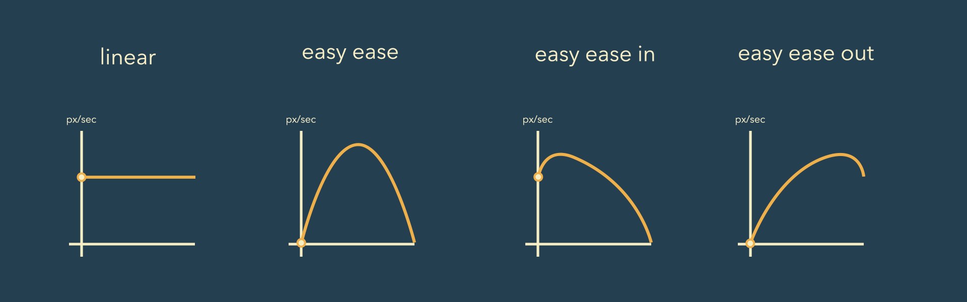 The graph editor also has buttons where you can apply any of those default easings to the selected keyframes with a single click. Just select the keyframes the want to ease (i.e. vertices of the speed graph) and then click any of the easing icons:
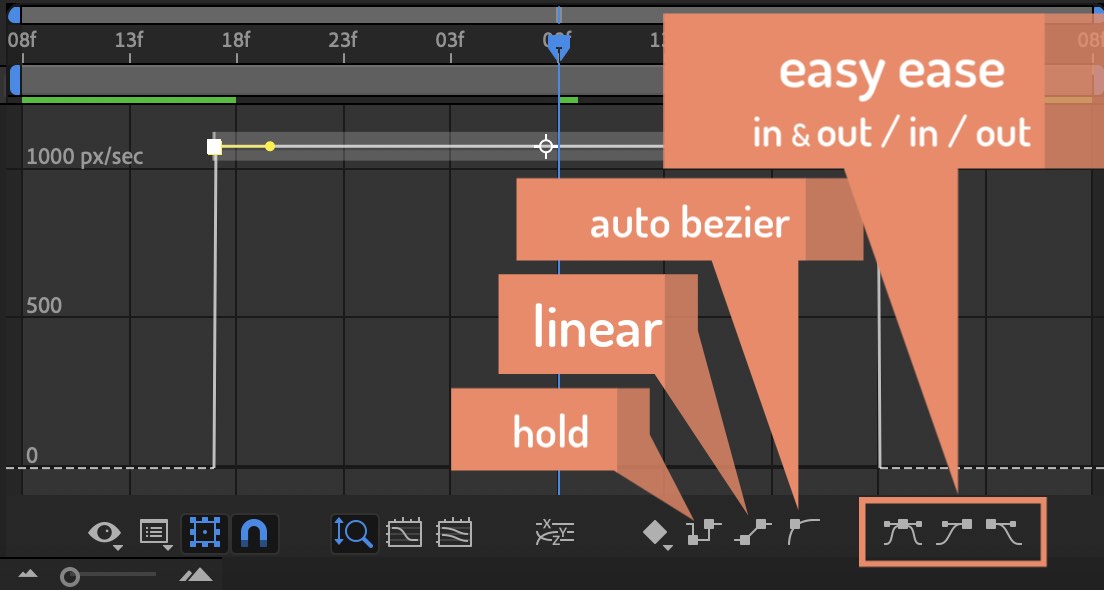 Hold and Auto Bezier are ‘fancier’ keyframe types, and we’ll cover these in the next section.
Now, take a look at the speed curves for Easy Ease In and Easy Ease Out. You’ll notice that Easy Ease In also always has a tiny bit of Ease Out, too: at the beginning, the speed curve goes up a bit before it starts to slow down. This is often unwanted, but barely noticeable. Now that you know the graph editor, you can edit your curves manually to fix these inaccuracies. When using Ease In, for example, just move the key at the start of the curve up until it no longer eases out.
Bouncing Balls and Constant Forces
Many motion designers have the intuition that speed curves must be smooth arcs, to create organic, eased motion. This is wrong. Motion paths are usually curved (see Section Arcs), but speed curves aren’t necessarily so. Let’s compare the speed curves that form a straight line to the default, bent speed curves of Easy Ease.
As we saw previously, a straight horizontal line corresponds to a movement with constant (linear) speed. In contrast to this, a straight line pointing upward accelerates over time - very similar to an Easy Ease Out. In fact, the easing is even more intense than that of the Easy Ease Out preset: It starts even slower and ends faster.
In terms of physics, a linear move is what happens when no force acts on the object at all - like a spaceship that doesn’t stop when the engines are turned off, but continues its movement with the same speed forever. The inclination of a speed curve shows the acceleration; so, in our spaceship example, this corresponds to how strong the ongoing jet propulsion is. A horizontal speed line has no inclination, so the jet engine is switched off. A straight speed line pointing upward has the same inclination everywhere, meaning the jet propulsion is running at a constant level. By contrast, the Easy Ease Out curve starts very steep and gets flatter and flatter over time. So for this curve, the jet propulsion is very strong at the beginning (steep curve) and then weakens over time.
So, horizontal lines correspond to no force at all, and other straight speed lines correspond to constant forces. An omnipresent constant force for animation is gravity. Bouncing balls, for example, are solely moved by gravity. Their speed curves look like this:
While the ball falls down, gravity accelerates it; while it’s moving up, gravity decelerates it. That’s why we have a zig zag pattern of straight lines. If the ball were 100% elastic and each bounce had the same height, the speed curve would look like a sawtooth wave. But in reality, some energy is lost with each bounce, so each peak is lower than the one before. In the speed graph, you can see this in the vertical lines at each of the peaks. These show that after each bounce, the ball is moving upward slower than it was moving downward right before the impact.
So, what does this mean for keyframing a bouncing ball? Well, to be fair I should first mention that I would never keyframe a bouncing ball manually. I developed the Throw 2D iExpression for all kinds of bouncing animations, which offers a very fast and playful way to literally drop or throw layers in your comp. The expression is based on a real physics simulation, and has real-time performance. However, keyframing a bouncing ball manually can be a very useful practical exercise.
One important lesson to learn: if you want to be physically accurate, there’s no guesswork necessary at all to get the easing right! Just make sure the speed curve has only straight lines, and that all of them have the same angle. If the animation still looks odd, it’s most likely not the easing but the distance between the keyframes that needs more adjustment. The controls of the graph editor are not really designed to create straight lines, but you also don’t have to be incredibly accurate. Keep in mind that animations don’t always need to be physically accurate. So, if you feel that a different speed curve looks better - go for it! Knowing what the ‘correct’ speed curve looks like is very helpful if your animation looks odd and you have no idea how you need to tweak it. But that shouldn’t stop you from experimenting - consider everything we say here about speed curves as hints, not strict rules.
Easy Ease is not good enough for Bouncing Balls
It seems to be conventional wisdom that bouncing ball animations can be created by simply adding an Easy Ease to the keyframes at the apex, and keeping the keyframes where the ball bounces on the ground linear. While this might be a simple solution, the result doesn’t really look good. Here’s a comparison of the simple Easy Ease approach and the correct easing with straight speed lines; to keep it simple, this time we’ve created a bounce with no decay.
The difference may be subtle, but I hope you’ll see that the part with straight speed lines looks more realistic. The one minute tutorial below shows how this animation was created - both the easy eased and the realistic examples. We make use of the separate dimensions feature in After Effects, which allows us to keyframe the x and y positions of a layer independently.
1D Speed Graphs & negative Speed
If you watched the tutorial above carefully, you may have been wondering why the speed graph had a different shape to the other bouncing ball animations we’ve seen before.
The reason is that with the separate dimensions option enabled, After Effects splits the 2D position property into two 1D properties for x and y. The speed graph for 1D properties has one small but important difference: for 1D properties, After Effects distinguishes whether the value increases or decreases, and when it decreases, the curve shows a negative speed. Let’s compare the 1D and the 2D variants of the speed curve for a bouncing ball: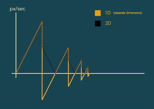
As I explained in the last section, the normal 2D position speed curve of a bouncing ball looks like the black, dotted line in this graph. But if you enable the ‘separate dimensions’ option for the layer, After Effects splits the position property into two separate properties for the x and y positions – the same animation then has a speed curve that looks like the orange line. In the parts where the ball falls (i.e. accelerates) the speed curves are identical, but in the parts where the ball moves upward, the 1D speed curve shows a negative speed (since moving upward means decreasing the y value). So, in these parts the 2D speed graph looks like a mirrored version of the 1D speed graph, where all the negative parts below the time axis are flipped upward to the positive area.
So, why is there no negative speed for 2D values? Well, for 2D values the speed is always measured along the motion path - and whether the movement goes upward, downward or in any other direction is just a question of the motion path itself, not the speed with which the layer travels along this path. A layer never travels backwards along the motion path, so its speed along the motion path is never negative.
The Aquarium
Do you feel that adjusting the speed graph is difficult or frustrating? Many people are confused by its behavior, in particular the fact that when you move one part of the curve down, another part moves up. If you’re struggling with this, the following tutorial might help.
In a nutshell, when you modify the speed graph, you’re not modifying a line, you are shaping the volume below the line, and this volume stays constant. And this can best be imagined by filling the volume with some balls.
Geek Alert
Mathematically, the speed curve is the derivative of the curve that plots the distance traveled vs time (or for 1D properties their value curve). So, the distance traveled is the integral of the speed curve. If you learned differential calculus in school, you might remember that the integral of a function corresponds to the area under the curve. That’s exactly what we have here – the distance travelled is the area under the speed curve. We’ve represented this area with balls, where each ball represents a part of the area, i.e. some part of the distance traveled (10 pixels, or 1 pixel, or whatever ball size you prefer). The more balls you stack on top of each other, the more the layer moves on this particular frame. Since the speed graph is only about timing, it will never change the motion path. The total distance traveled (and consequently the number of balls) will never change.
A Subtle (Advanced) Example
When you adjust easing curves, the differences are often subtle. If you don’t have much experience, the following three variants might look identical to you.
The movements for the left and right dot have exactly the same timing – their speed curves are identical – so let’s just look at one of them. All three variants start with an ease out keyframe and end with a linear keyframe (we want to start softly, but make the crash at the end abrupt). But the middle keyframe where the dots change direction is different for all three variants: it’s linear for the first variant, easy eased for the second and has a custom speed curve for the third one.
If all three of these look identical to you, don’t worry – we’re here to train your brain (see Brains Simplify Reality). Focus only on the left dot in the first example, and try to figure out how the speed changes around the turning point of the move. It’s an abrupt change – it goes full speed towards the top left, then abruptly changes to move in the opposite direction.
In contrast, the second variant decelerates a little when approaching the turning point, and accelerates again after the turn. The turn feels softer. You can see this in the graph editor, since the speed goes towards zero when approaching the turning point and then slowly goes up again after the turn. By contrast, in the linear graph it doesn’t touch the zero line and also abruptly (vertical line) jumps to a much higher speed at the turn.
For the third variant, I exaggerated the easing that was already present in the second variant – the move towards the turning point starts very slow, then gets very fast, and then slows down again a lot when it approaches the turning point.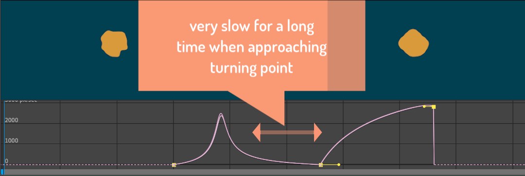 As a result, the layer seems to pause slightly around the turning point, as if taking a deep breath before the main action.
These differences are subtle, but they make a difference. The eased variants are more plausible in terms of physics, but they also feel better. If you look at the speed curves in the graph editor, you can assess the motion much better and more precisely than you could by just looking at the animation itself.

Create complex expression-driven templates, character rigs, shape animations and more without writing any code!

Streamline your live 3D pipeline between Cinema 4D and After Effects CC. Quickly toggle between the live pipeline and rendered proxy files.